One of the deliverable features of this project is an integration with the CKAN.

To implement this the harvester framework for CKAN was installed into an instance of CKAN and then the data.bris havester plugin has been used to harvest the location and the META data of datasets.

From the systems point of view all that is required of it is for a RDF file to be generated which lists the META data for that dataset. This META data can include a set of tags.

It's these tags which are being used to allow for the discovery of other datasets. If the system generates the same tags for two different datasets they will be related and hence these tags will facilitate discovery.

The following are a few screenshots of the system in place. Currently they are showing the tags for columns in a dataset but it'll show the dataset level tags in the same way.

In future imports the automatically generated tags will have some sort of text appended to them to show that they were generated by this system and so would allow them to co-exist with user curated tags.

Within a dataset there are two types of variables "Discrete" and "Continuous". The first of these are simple and are binary in nature. The presence of a "/" can be answered simply as a True or False.

However if the tagging system was limited to only these variables a lot of information that can be extracted for the system will be ignored.

Because of this a methodology for incorporating continuous variables into the network must be identified.

There are two different general approaches to mixing both discrete and continuous variables into a network as described in [1]. These are the discretising of the continuous variable into a set of discrete variables representing ranges and the second is to keep them as continuous variables and introduce new techniques to handle the situation such as the conditional Gaussian (CG) distribution or the Mixture of Truncated Exponentials (MTE) model both these methods are described in [1].

Discretising of Continuous Variables

This approach to incorporating continuous variables into a Bayesian network is to turn continuous variables into discrete ones. The basic approach to this is to choose a set of threshold values which partition the continuous variable into a set of discrete variables [2] which can then be incorporated into a traditional bayesian network.

The CG Method

The CG method build a hybrid network with the state space defined by the following

Where y represents the discrete variables and z representes the continuous. It can then be modeled using the Multivariate Gaussian distribution

The CG method however has a limitation in that a discrete node cannot have a continuous parent. This limits the possible structure of the graph and as the optimal or even desired structure of the graph is unknown this limitation is non desirable.

The MTE Model

The MTE model is described in full and is summarised in [1] by stating "Since discretization is equivalent to approximating a target density by a mixture of uniforms, the accuracy of the final model could be increased if, instead of uniforms, other distributions with higher fitting power were used.".

The MTE model is also able to have continuous parents unlike the CG method [1].

To understand the need for multiple bounded variables to represent one variable one must look at the data.

A histogram of example salary data with 10 buckets.

A histogram of example salary data with 100 buckets.

The two histograms have been generated on some example salary data drawn from a sample of datasets from data.gov.uk.

When the histogram is generated with only 10 buckets it can be seen there is a single mode and that the data could approximated quite well with a normal distribution. However when the granularity of the histogram is increased so that it has 100 buckets it can be seen the data appears to be bimodal. This makes sense when looking at the data with context. Whilst salaries can be any value they tend to gravitate towards a standard value in a given range and so for each range the data will likely be normally distributed.

The Dataset Tagging Project

Within this post various different approaches to dealing with continuous data has been analysed. The two promising approaches seem to be the simple discretisation of continuous variables and the MTE approach. Out of these two the MTE model would seem to be the best approach however at this point in time it is unclear if it would be practical to integrate this with the PYMC library which is being used to implement the belief network.

[1] Cobb, Barry R., Rafael Rumı, and Antonio Salmerón. "Bayesian Network Models with Discrete and Continuous Variables."

[2] Friedman, Nir, and Moises Goldszmidt. "Discretizing continuous attributes while learning Bayesian networks."

The Models

As previously discussed PYMC uses models to represent the graph structure on which it can do sampling upon.

These models are contained in a python source file. When one wants to use a model they are imported and passed into PYMC.

The Problem

The problem with this approach revolves around when one wants to change the model slightly or update the learnt probabilities. Manually editing it is of course inefficient. Further difficulty is introduced when we want to change the graph structure in multiple subsystems.

The Solution

The solution chosen was to automatically generate the python source files that make up the models. Whilst this is not the immediately obvious solution any other potential workaround look to be possibly even more painful.

The generator imports the graph from a file which is made up of the simple graph language that has been previously discussed. In addition to this the generator takes an input of observed variables.

The graph is then passed. For each node a node in the model is created, similarly a probability function is created in accordance to the relationships defined in the graph definition and from the stored CPT data that was gathered during the training stage.

If a node is observed (identified by the passed list of observed variables) this will be marked in the model as well.

By dynamically allowing the observed nodes to be set in code it allows for the system to generate a model to answer questions like P(X|A,C).

When the model has been created all that needs to be done is to reload it and then to sample from it.

Simple to explain, annoying to get working.

Over the last week rapid progress is being made moving towards an initial test of the system on an artificial dataset.

This process has involved integrating various sub-systems that have been written so far with external libraries that have been adopted as well as writing some new code.

The current architectural layout is roughly as follows.

1. Graph language
2. CPT Learner
3. Model Generation
4. Observer
5. Sampler

Graph Language

This a small and simple plain text representation of the graph structure. It serves as a standard representation of the graph that can be transcribed into the format required by each of the subsystems. At a later date this will be auto generated through machine learning techniques.

CPT Learner

This subsystem has evolved from the code discussed previously in this blog. It loads in the graph from the graph language and represents it in a network. Training data is then passed with this graph structure in mind and CPTs for each node are generated. These are stored at the end of the training process using the Python 'pickle' library to serialise the  CPT itself.

Model Generation

PYMC utilises models to perform calculations upon (see Adventures with PYMC for more details). To make this possible the model generation system combines the graph structure from the graph language and the learnt CPTs stored in pickle files to generate a python file that represents the model for PYMC to use. One can also pass observed variables into the model.

Observer

The observer looks through a dataset and identifies observed nodes in the data that correspond to nodes the graph structure. These are then passed into the aforementioned model generation system.

Sampler

With the model is created it can now be sampled. This uses the PYMC library. The result of the sampling allows the probability of each node to be extracted.

Further details of some of these stages will be discussed in subsequent blog posts.

In the last post on this blog various python libraries were listed as candidates for use in the data tagging project. After some further research 'pymc' has been selected.

The library is hosted on github at - https://github.com/pymc-devs/pymc

It is a feature rich library and looks to be a good fit for the project. The last couple of weeks have involved becoming acquainted with the library and attempting to implement the functionality which had existed with the custom Bayesian network code. Whilst throwing away progress is always painful the investment is looking to be a good one.

The following is a whistle stop tour which includes creating a Bayesian Network with PYMC and then querying data from it.

Once again the example network and data being used is the 'sprinkler' example taken from the wikipedia page.

Shown below is just a reminder of the layout of the network and the CPTs associated with the nodes.

The sprinkler network

T     F  
*********
0.2   0.8   

A   *   T      F   
*******************
F   *   0.4    0.6    
T   *   0.1    0.99   

B   A   *   T      F   
***********************
F   F   *   0.0    1.0    
F   T   *   0.8    0.2    
T   F   *   0.9    0.1    
T   T   *   0.99   0.01

Setting up the network

To create the internal representation of the network is relatively simple.

Defining a simple node

To define a simple node with no conditions (such as node A) is simple.

nodename = pymc.Bernoulli('nodename', 0.2)

Defining a conditional node

When there is conditions (such as node b) it is still quite simple. This time one must first setup the conditional probability.

probNodeName = mc.Lambda('probNodeName', lambda conditionalNode = conditionalNode: pylab.where(conditionalNode, 0.01, 0.4))

The next step is to create the node using the conditional probability defined above. Here it is being modeled using the Bernoulli distribution, however there is support for a range of distributions.

nodename = mc.Bernoulli('nodename', probNodeName)

P( A | C)

This is one of the most basic questions to answer with a Bayesian network. With the network setup it is simple to answer this question.

First we must set C as observed. To do this the following parameters are added during the node setup.

value=[1.0], observed=True

The network is then sampled. In this example the Markov chain Monte Carlo sampling technique is used. This is down with the following code were model is the model that contains the network.

model.sample(60000)

When this has been completed the answer to the above question can be simply read out of the graph.

m.nodename.stats()['mean']

Which gives an answer of 0.32658333333333334 or ~= 32.65% which is not 100% accurate but would improve with further sampling.

To this point in the project the Bayesian Networks have been implemented without using a library. NetworkX has been used for representing the underlying graph structure but everything from that point up has been implemented by hand.

In an aim to follow the "pythonic way" I have begun looking into existing libraries to implement the Bayesian Network. The goal of this investigation is that that using an existing package would decrease the development time of this project.

After some initial research I have created a short list of the various libraries that will be considered in greater depth.

PBNT – Python Bayesian Network Toolbox

http://pbnt.berlios.de/

Pebl - Python Environment for Bayesian Learning

https://github.com/abhik/pebl

PyBayes

https://github.com/strohel/PyBayes

Orange

http://orange.biolab.si/

Pymc

https://github.com/pymc-devs/pymc

As previously discussed Bayesian Belief Networks are being used within this project to perform high level type inference. To do this inference will be performed using the constructed graph.

However before inference can take place it is first necessary to train the Bayesian Network.

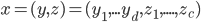
The graph being used for this initial test contains the following nodes:

LatLon, £, $, Int, Money, Float, Location, Number, €, String, PostCode,
Date, Name

It can be represented graphically as follows:

The labeling of data for training is implemented in two ways.

The first method uses the basic type inference system as previously described. For each piece of data each data type is considered and if the method returns true it can be determined that a positive observation for that datatype has occurred.

The second of method involves the hand labeling of data columns. When the caching system (as previously described) reads in the data it produces an additional text file that stores the column labels and allows for the columns to be labeled by hand. When the cached data is read in for processing at a later date the labels are loaded into to the data structure that contains the data.

When the training method is called it can then look to see if there is a label for this column and hence for every piece of data in that column mark a positive observation for that datatype.

Storing the Evidence

Currently conditional probability tables (CPTs) are used to store the training data. This has the limitation in that only features that are boolean in nature, such as "is it raining?", can be represented. Meaning continuous data, such as quantity of rainfall, can not be represented at this time.

With this said the CPTs are represented internally in the following way.

For each row in the CPT there is the following:

[Array of dependency nodes], [Array representing the boolean values of the dependencies], [Positive Observations, Total Observations]

Intuitively it can be seen that a probability can be derived by the following,

P = Positive Observations/Total Observations

And similarly the probability of it not being a particular type can be derived by the following,

¬P = 1-Positive Observations/Total Observations

The probabilities are not stored as a float internally for efficiency reasons.

The number of rows in a CPT is equal to to 2^(# of dependency nodes). To derive all the combinations of True and False values for all of these rows is simple. One simply counts from 0 to the number of rows and converts the integer number to a binary string and then converts it to an array of True and Falses.

When the training system identifies a positive observation it must be attributed to the correct row within the CPT. To do this it traverses all the nodes linked into the current node, for each it get a True or False value which represent their state in regards to this piece of data. These are assembled into an array matching the format of that within the CPT. The CPT is then traversed until a matching array is found and hence the correct row has been found. The positive observation is then attributed to this row.

Output

Please note that 1. the training set is very limited and 2. the basic type inference is not complete so the actual values here are inaccurate but it serves to demonstrate the training system.

LatLon
Int   *   Present   Observed
****************************
F     *   0     598   
T     *   0     12    

£
Present   Observed
******************
0     610   

$
Present   Observed
******************
0     610   

Int
Present   Observed
******************
12    610   

Money
£   Number   $   €   *   Present   Observed
*******************************************
F     F     F     F        *   61       610      
F     F     F     T        *   0        0        
F     F     T     F        *   0        0        
F     F     T     T        *   0        0        
F     T     F     F        *   0        0        
F     T     F     T        *   0        0        
F     T     T     F        *   0        0        
F     T     T     T        *   0        0        
T     F     F     F        *   0        0        
T     F     F     T        *   0        0        
T     F     T     F        *   0        0        
T     F     T     T        *   0        0        
T     T     F     F        *   0        0        
T     T     F     T        *   0        0        
T     T     T     F        *   0        0        
T     T     T     T        *   0        0

Float                                                                                                                                                                                                                                                                 
Present   Observed
******************
73    610   

Location
LatLon   PostCode   *   Present    Observed
*******************************************
F       F          *   0          610        
F       T          *   0          0          
T       F          *   0          0          
T       T          *   0          0          

Number
Int   Float   *   Present   Observed
************************************
F    F       *   171     537     
F    T       *   0       61      
T    F       *   0       0       
T    T       *   12      12      

€
Present   Observed
******************
0     610   

String
Present   Observed
******************
610   610   

PostCode
String   *   Present   Observed
*******************************
F        *   0        0        
T        *   0        610      

Date
Int   *   Present   Observed
****************************
F     *   61    598   
T     *   0     12    

Name
String   *   Present   Observed
*******************************
F        *   0        0        
T        *   0        610

There has been lots of progress today but sadly nothing major to write up.

However I've been hand crafting the Bayesian network which has led to a more interesting example of the graph output which can be shown.

Hopefully something more interesting will follow soon.

The Bayesian Belief Networks used in the tagging system are represented as graphs. In particular they are directed acyclic graphs (DAGs).

Within this project the graphing system will have various requirements placed upon it.

• Representation of the each nodes random variable.
• Ability to render out a visual representation of the graph (for use in the dissertation and for debugging purposes).
• Storing of additional information such as a nodes name.

The initial implementation of this within the project was a bespoke system created from scratch, whilst this worked, the visual representation requirement would have taken extensive work to be of high enough quality for use. To resolve this it was decided to take advantage of the extensive range of packages available for python.

As a result of this research the current implementation is based upon the NetworkX python package which was created by the Los Alamos National Laboratory. It is a package designed for the creation and manipulation of network/graphs. Importantly it has rich support for rendering of the represented graph in a visual form when combined with the matplotlib python package.

In this new implementation I have implemented a method to represent a conditional probability table (CPT), the CPTs are attached as attributes to the nodes in the graph and will be used later for the inference process. As discussed before these need to be able to be rendered out in a human readable form, for use in the dissertation and for debugging purposes. A function has be created to facilitate this.

The result of this work is shown below. The example CPT values and the simple graph structure have been taken from the example in the wikipedia page on Bayesian Networks. They are purely for demonstration purposes and will have no relevance to the actual project.

A simple Bayesian network.

And the following is the human readable form of the the CPTs.

T     F  
*********
0.2   0.8   

A   *   T      F   
*******************
F   *   0.4    0.6    
T   *   0.1    0.99   

B   A   *   T      F   
***********************
F   F   *   0.0    1.0    
F   T   *   0.8    0.2    
T   F   *   0.9    0.1    
T   T   *   0.99   0.01

Whilst the example shown here is simple, the implementation can scale to a much larger graph and allows for the performance of inference from the graph represented.

Summary

• Graph representation has been implemented (once without external packages and once with NetworkX).
• Rendering to human form of the graph and data contained within it.

Next

Write the code to perform the actual inference from the Bayesian network represented in this work.

The end result of this project is to hypothesise tags for each dataset stored within a CKAN instance. As part of this it is necessary to look at the data within every dataset. To do this one must first understand the type of data that is being looked at, to understand the primitive types that each piece of data is.

Primitive Type Inference System

Any one who is familiar with basic programming understands the basic concept of a type. "String", "Float" and "Integers" are all well known examples of this. In addition to this, to aid  in the later processing of the data it useful to provide as much information as possible so additional type have been added to these well known datatypes. Currently these are "Currency" and "Date" but more will be added to the system as time goes on.

Hierarchal Data Types

At this point the hierarchal nature of datatypes can already be seen. For example:

Date -> String
Currency -> Float -> String or Currency -> Integer -> String or Currency -> String

(Where the left most datatype is the highest level.)

The next iteration of this system will represent these, however as is stands at the moment they are not. It does however describe a challenge to the inference system. If we were to firstly consider if a value is a string the answer will always be true, as anything that we can load in from a file will be able to be represented as a string, it is after all the type that value be read from the file as.

Implementation

After doing some cursory reading in this area it was decided to attempt a very simplistic prototype to better understand the problem.

To do this a range of methods were created that are able to state if a value is of a particular type. Each one of these have been implemented in different ways ranging from regular expressions (dates) to simply attempting a cast and seeing if it succeeds (integers).

By taking into consideration the hierarchal nature of types as discussed above the system then can simply test a value against each of the decider methods in order from highest level type to lowest and return the value type as soon as on of the methods returns True.

Summary

• Additional type information can be used to help later processing.
• Type data can be represented in hierarchal fashion.
• A simplistic type inference implementation.