Within a dataset there are two types of variables "Discrete" and "Continuous". The first of these are simple and are binary in nature. The presence of a "/" can be answered simply as a True or False.
However if the tagging system was limited to only these variables a lot of information that can be extracted for the system will be ignored.
Because of this a methodology for incorporating continuous variables into the network must be identified.
There are two different general approaches to mixing both discrete and continuous variables into a network as described in [1]. These are the discretising of the continuous variable into a set of discrete variables representing ranges and the second is to keep them as continuous variables and introduce new techniques to handle the situation such as the conditional Gaussian (CG) distribution or the Mixture of Truncated Exponentials (MTE) model both these methods are described in [1].
Discretising of Continuous Variables
This approach to incorporating continuous variables into a Bayesian network is to turn continuous variables into discrete ones. The basic approach to this is to choose a set of threshold values which partition the continuous variable into a set of discrete variables [2] which can then be incorporated into a traditional bayesian network.
The CG Method
The CG method build a hybrid network with the state space defined by the following
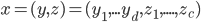
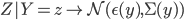
Where y represents the discrete variables and z representes the continuous. It can then be modeled using the Multivariate Gaussian distribution
The CG method however has a limitation in that a discrete node cannot have a continuous parent. This limits the possible structure of the graph and as the optimal or even desired structure of the graph is unknown this limitation is non desirable.
The MTE Model
The MTE model is described in full and is summarised in [1] by stating "Since discretization is equivalent to approximating a target density by a mixture of uniforms, the accuracy of the final model could be increased if, instead of uniforms, other distributions with higher fi tting power were used.".
The MTE model is also able to have continuous parents unlike the CG method [1].
To understand the need for multiple bounded variables to represent one variable one must look at the data.

A histogram of example salary data with 10 buckets.

A histogram of example salary data with 100 buckets.
The two histograms have been generated on some example salary data drawn from a sample of datasets from data.gov.uk.
When the histogram is generated with only 10 buckets it can be seen there is a single mode and that the data could approximated quite well with a normal distribution. However when the granularity of the histogram is increased so that it has 100 buckets it can be seen the data appears to be bimodal. This makes sense when looking at the data with context. Whilst salaries can be any value they tend to gravitate towards a standard value in a given range and so for each range the data will likely be normally distributed.
The Dataset Tagging Project
Within this post various different approaches to dealing with continuous data has been analysed. The two promising approaches seem to be the simple discretisation of continuous variables and the MTE approach. Out of these two the MTE model would seem to be the best approach however at this point in time it is unclear if it would be practical to integrate this with the PYMC library which is being used to implement the belief network.
[1] Cobb, Barry R., Rafael Rumı, and Antonio Salmerón. "Bayesian Network Models with Discrete and Continuous Variables."
[2] Friedman, Nir, and Moises Goldszmidt. "Discretizing continuous attributes while learning Bayesian networks."